Examples
Note
For a full description of the available functionality, see the API Reference section.
The main binding of CLASS is available to users in the classylss.binding
module. To start, we shall make the necessary imports and print out the
classylss version and CLASS version:
In [1]: import classylss
In [2]: import classylss.binding as CLASS
In [3]: print("classylss version = ", classylss.__version__)
classylss version = 0.2.6
In [4]: print("CLASS version = ", classylss.class_version)
���������������������������CLASS version = 2.6.1
Initializing the CLASS engine
Users must first initialize the CLASS engine, optionally passing in a dictionary
of parameters. If no parameters are passed, the default CLASS parameters are used.
This can be done using the classylss.binding.ClassEngine class as
In [5]: engine = CLASS.ClassEngine({'H0':70, 'Omega_m':0.31})

In [6]: default_engine = CLASS.ClassEngine() # default parameters
Loading parameters from file
Users can use the classylss.load_ini() function to load parameters
from a CLASS .ini file into a dictionary. For example, we can load
the concise.ini
parameter file from the CLASS GitHub and use these parameters to initialize
our ClassEngine:
In [7]: params = classylss.load_ini('concise.ini')

In [8]: print(params)
{'H0': '72.', 'omega_b': '0.0266691', 'omega_cdm': '0.110616', 'reio_parametrization': 'reio_camb', 'z_reio': '10.', 'output': 'tCl', 'A_s_ad': '2.3e-9', 'n_s_ad': '1.', 'l_scalar_max': '2500'}

In [9]: engine = CLASS.ClassEngine(params)
Loading precision parameters from file
We can also pass in precision parameters that have been loaded from file
using the classylss.load_precision() function. For example, we can load
the pk_ref.pre
parameter file from the CLASS GitHub:
In [10]: pre_params = classylss.load_precision('pk_ref.pre')

In [11]: print(pre_params)
{'tol_ncdm_bg': 1e-10, 'recfast_Nz0': 100000, 'tol_thermo_integration': 1e-05, 'recfast_x_He0_trigger_delta': 0.01, 'recfast_x_H0_trigger_delta': 0.01, 'evolver': 0, 'k_min_tau0': 0.002, 'k_max_tau0_over_l_max': 3.0, 'k_step_sub': 0.015, 'k_step_super': 0.0001, 'k_step_super_reduction': 0.1, 'start_small_k_at_tau_c_over_tau_h': 0.0004, 'start_large_k_at_tau_h_over_tau_k': 0.05, 'tight_coupling_trigger_tau_c_over_tau_h': 0.005, 'tight_coupling_trigger_tau_c_over_tau_k': 0.008, 'start_sources_at_tau_c_over_tau_h': 0.006, 'l_max_g': 50, 'l_max_pol_g': 25, 'l_max_ur': 150, 'l_max_ncdm': 50, 'tol_perturb_integration': 1e-06, 'perturb_sampling_stepsize': 0.01, 'radiation_streaming_approximation': 2, 'radiation_streaming_trigger_tau_over_tau_k': 240.0, 'radiation_streaming_trigger_tau_c_over_tau': 100.0, 'ur_fluid_approximation': 2, 'ur_fluid_trigger_tau_over_tau_k': 50.0, 'ncdm_fluid_approximation': 3, 'ncdm_fluid_trigger_tau_over_tau_k': 51.0, 'tol_ncdm_synchronous': 1e-10, 'tol_ncdm_newtonian': 1e-10, 'l_logstep': 1.026, 'l_linstep': 25, 'hyper_sampling_flat': 12.0, 'hyper_sampling_curved_low_nu': 10.0, 'hyper_sampling_curved_high_nu': 10.0, 'hyper_nu_sampling_step': 10.0, 'hyper_phi_min_abs': 1e-10, 'hyper_x_tol': 0.0001, 'hyper_flat_approximation_nu': 1000000.0, 'q_linstep': 0.2, 'q_logstep_spline': 20.0, 'q_logstep_trapzd': 0.5, 'q_numstep_transition': 250, 'transfer_neglect_delta_k_S_t0': 100.0, 'transfer_neglect_delta_k_S_t1': 100.0, 'transfer_neglect_delta_k_S_t2': 100.0, 'transfer_neglect_delta_k_S_e': 100.0, 'transfer_neglect_delta_k_V_t1': 100.0, 'transfer_neglect_delta_k_V_t2': 100.0, 'transfer_neglect_delta_k_V_e': 100.0, 'transfer_neglect_delta_k_V_b': 100.0, 'transfer_neglect_delta_k_T_t2': 100.0, 'transfer_neglect_delta_k_T_e': 100.0, 'transfer_neglect_delta_k_T_b': 100.0, 'neglect_CMB_sources_below_visibility': 1e-30, 'transfer_neglect_late_source': 3000.0, 'l_switch_limber': 40.0, 'accurate_lensing': 1, 'num_mu_minus_lmax': 1000.0, 'delta_l_max': 1000.0}

# default cosmo params + precision params
In [12]: high_pre_engine = CLASS.ClassEngine(pre_params)
Using the main CLASS modules
The Background module
The background module in CLASS computes
background cosmology quantities, e.g., distances, as a function of redshift.
It also provides access to the parameters of the specified cosmological model.
In classylss, the classylss.binding.Background object provides
an interface to this module.
# initialize the background module
In [13]: bg = CLASS.Background(engine)
# print out some cosmological parameters
In [14]: print("h = ", bg.h)
h = 0.72
In [15]: print("Omega0_m = ", bg.Omega0_m)
����������Omega0_m = 0.2648246527777778
In [16]: print("Omega0_lambda = ", bg.Omega0_lambda)
�����������������������������������������Omega0_lambda = 0.735094642951158
In [17]: print("Omega0_r = ", bg.Omega0_r)
����������������������������������������������������������������������������Omega0_r = 8.070427106422706e-05
In [18]: print("Omega0_k = ", bg.Omega0_k)
��������������������������������������������������������������������������������������������������������������Omega0_k = 0.0
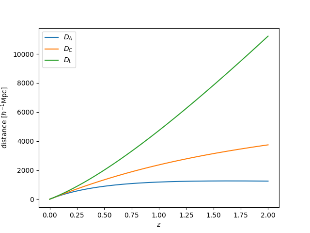
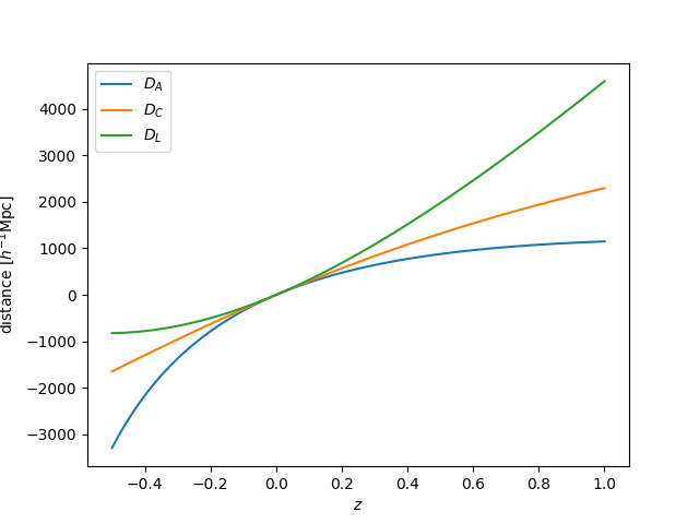
Distances
We can plot distances measures as a function of redshift using:
In [19]: import numpy as np
In [20]: from matplotlib import pyplot as plt
In [21]: z = np.linspace(0., 2., 1024)
In [22]: plt.plot(z, bg.angular_diameter_distance(z), label=r"$D_A$")
Out[22]: [<matplotlib.lines.Line2D at 0x7fc47c08ed68>]
In [23]: plt.plot(z, bg.comoving_distance(z), label=r"$D_C$")
�������������������������������������������������������Out[23]: [<matplotlib.lines.Line2D at 0x7fc47c0996d8>]
In [24]: plt.plot(z, bg.luminosity_distance(z), label=r"$D_L$")
��������������������������������������������������������������������������������������������������������������Out[24]: [<matplotlib.lines.Line2D at 0x7fc47c099be0>]
# save
In [25]: plt.legend()
���������������������������������������������������������������������������������������������������������������������������������������������������������������������Out[25]: <matplotlib.legend.Legend at 0x7fc47c0996a0>
In [26]: plt.xlabel(r"$z$")
���������������������������������������������������������������������������������������������������������������������������������������������������������������������������������������������������������������������������Out[26]: Text(0.5,0,'$z$')
In [27]: plt.ylabel(r"distance $[h^{-1} \mathrm{Mpc}]$")
������������������������������������������������������������������������������������������������������������������������������������������������������������������������������������������������������������������������������������������������������Out[27]: Text(0,0.5,'distance $[h^{-1} \\mathrm{Mpc}]$')
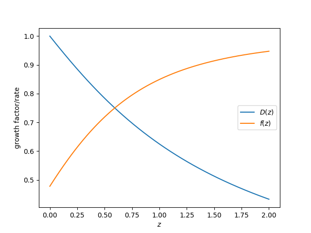
Linear growth evolution
The linear growth factor and growth rate can be computed as:
In [28]: z = np.linspace(0., 2., 1024)
In [29]: plt.plot(z, bg.scale_independent_growth_factor(z), label=r"$D(z)$")
Out[29]: [<matplotlib.lines.Line2D at 0x7fc47124fbe0>]
In [30]: plt.plot(z, bg.scale_independent_growth_rate(z), label=r"$f(z)$")
�������������������������������������������������������Out[30]: [<matplotlib.lines.Line2D at 0x7fc47c03d160>]
# save
In [31]: plt.legend()
��������������������������������������������������������������������������������������������������������������Out[31]: <matplotlib.legend.Legend at 0x7fc47d088e10>
In [32]: plt.xlabel(r"$z$")
��������������������������������������������������������������������������������������������������������������������������������������������������������������������Out[32]: Text(0.5,0,'$z$')
In [33]: plt.ylabel("growth factor/rate")
�����������������������������������������������������������������������������������������������������������������������������������������������������������������������������������������������Out[33]: Text(0,0.5,'growth factor/rate')
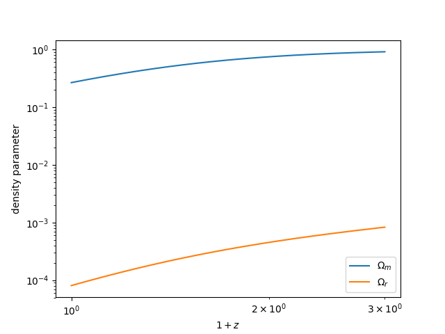
Density parameter evolution
The density parameters \(\Omega\) can be computed as a function of redshift for various species:
In [34]: z = np.linspace(0., 2., 1024)
In [35]: plt.loglog(1+z, bg.Omega_m(z), label=r"$\Omega_m$")
Out[35]: [<matplotlib.lines.Line2D at 0x7fc47c01c358>]
In [36]: plt.loglog(1+z, bg.Omega_r(z), label=r"$\Omega_r$")
�������������������������������������������������������Out[36]: [<matplotlib.lines.Line2D at 0x7fc47c05eb70>]
# save
In [37]: plt.legend()
��������������������������������������������������������������������������������������������������������������Out[37]: <matplotlib.legend.Legend at 0x7fc471290630>
In [38]: plt.xlabel(r"$1+z$")
��������������������������������������������������������������������������������������������������������������������������������������������������������������������Out[38]: Text(0.5,0,'$1+z$')
In [39]: plt.ylabel("density parameter")
�������������������������������������������������������������������������������������������������������������������������������������������������������������������������������������������������Out[39]: Text(0,0.5,'density parameter')
Setting a_max
Quantities in the background module can also be computed for \(a > 1\) by
setting the a_max parameter. Below, we compute the same distance calculations
up to \(a_\mathrm{max}=2\):
In [40]: a_max = 2.0
In [41]: cosmo = CLASS.ClassEngine({'a_max':a_max})
In [42]: bg = CLASS.Background(cosmo)
In [43]: z = np.linspace(1/a_max-1, 1, 1024)
In [44]: plt.plot(z, bg.angular_diameter_distance(z), label=r"$D_A$")
Out[44]: [<matplotlib.lines.Line2D at 0x7fc47123bf98>]
In [45]: plt.plot(z, bg.comoving_distance(z), label=r"$D_C$")
�������������������������������������������������������Out[45]: [<matplotlib.lines.Line2D at 0x7fc47123bb38>]
In [46]: plt.plot(z, bg.luminosity_distance(z), label=r"$D_L$")
��������������������������������������������������������������������������������������������������������������Out[46]: [<matplotlib.lines.Line2D at 0x7fc4712206d8>]
# save
In [47]: plt.legend()
���������������������������������������������������������������������������������������������������������������������������������������������������������������������Out[47]: <matplotlib.legend.Legend at 0x7fc47114f048>
In [48]: plt.xlabel(r"$z$")
���������������������������������������������������������������������������������������������������������������������������������������������������������������������������������������������������������������������������Out[48]: Text(0.5,0,'$z$')
In [49]: plt.ylabel(r"distance $[h^{-1} \mathrm{Mpc}]$")
������������������������������������������������������������������������������������������������������������������������������������������������������������������������������������������������������������������������������������������������������Out[49]: Text(0,0.5,'distance $[h^{-1} \\mathrm{Mpc}]$')
The Spectra module
The spectra module in CLASS computes
linear density and velocity transfer functions, as well as the linear
and nonlinear density power spectra. In classylss, the
classylss.binding.Spectra object provides an interface to this module.
# initialize with proper output
In [50]: cosmo = CLASS.ClassEngine({'output': 'dTk vTk mPk', 'non linear': 'halofit', 'P_k_max_h/Mpc' : 20., "z_max_pk" : 100.0})

In [51]: sp = CLASS.Spectra(cosmo)
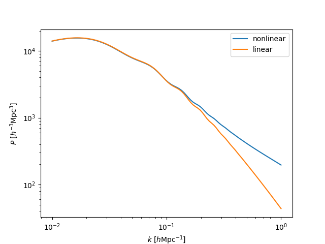
The linear and nonlinear power spectra
We can compute the nonlinear and linear power spectra at the desired redshifts and wavenumbers using:
In [52]: z = 0.5
In [53]: k = np.logspace(-2, 0, 100)
# nonlinear power
In [54]: pk_nl = sp.get_pk(k=k, z=z)
# linear power
In [55]: pk_lin = sp.get_pklin(k=k, z=z)
In [56]: plt.loglog(k, pk_nl, label='nonlinear')
Out[56]: [<matplotlib.lines.Line2D at 0x7fc4711e12e8>]
In [57]: plt.loglog(k, pk_lin, label='linear')
�������������������������������������������������������Out[57]: [<matplotlib.lines.Line2D at 0x7fc4710f0e48>]
# save
In [58]: plt.legend()
��������������������������������������������������������������������������������������������������������������Out[58]: <matplotlib.legend.Legend at 0x7fc471105390>
In [59]: plt.xlabel(r"$k$ $[h\mathrm{Mpc}^{-1}]$")
��������������������������������������������������������������������������������������������������������������������������������������������������������������������Out[59]: Text(0.5,0,'$k$ $[h\\mathrm{Mpc}^{-1}]$')
In [60]: plt.ylabel(r"$P$ $[h^{-3} \mathrm{Mpc}^3]$")
�����������������������������������������������������������������������������������������������������������������������������������������������������������������������������������������������������������������������Out[60]: Text(0,0.5,'$P$ $[h^{-3} \\mathrm{Mpc}^3]$')
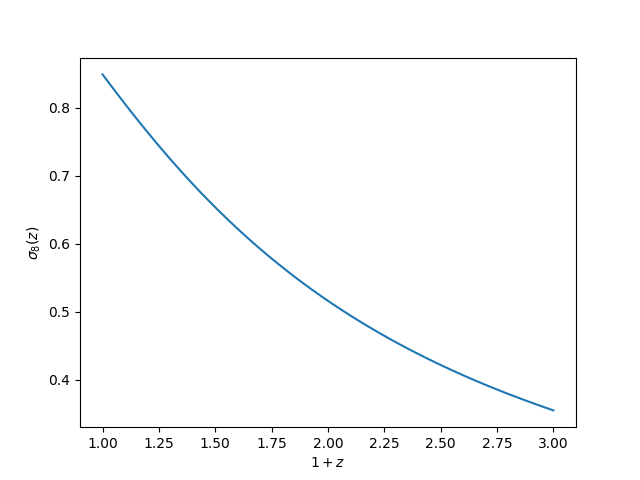
The evolution of \(\sigma_8\)
The evolution of the perturbation amplitude \(\sigma_8\) can be computed using:
In [61]: z = np.linspace(0., 2., 1024)
In [62]: plt.plot(1 + z, sp.sigma8_z(z))
Out[62]: [<matplotlib.lines.Line2D at 0x7fc47107c8d0>]
# save
In [63]: plt.xlabel(r"$1+z$")
�������������������������������������������������������Out[63]: Text(0.5,0,'$1+z$')
In [64]: plt.ylabel(r"$\sigma_8(z)$")
������������������������������������������������������������������������������������Out[64]: Text(0,0.5,'$\\sigma_8(z)$')
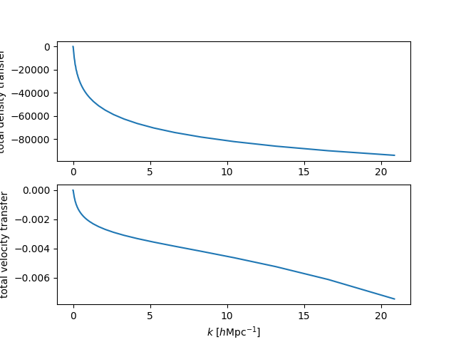
Density and velocity transfers
We can compute the transfer functions in CLASS units for density, velocity and
\(\phi\) in CLASS units, using get_transfer():
# transfer at z=0
In [65]: transfer = sp.get_transfer(z=0)
In [66]: print(transfer.dtype.names)
('k', 'd_g', 'd_b', 'd_cdm', 'd_ur', 'd_tot', 'phi', 'psi', 't_g', 't_b', 't_ur', 't_tot')
In [67]: plt.subplot(211)
�������������������������������������������������������������������������������������������Out[67]: <matplotlib.axes._subplots.AxesSubplot at 0x7fc470fed8d0>
In [68]: plt.plot(transfer['k'], transfer['d_tot'])
��������������������������������������������������������������������������������������������������������������������������������������������������������������Out[68]: [<matplotlib.lines.Line2D at 0x7fc4710f29b0>]
In [69]: plt.ylabel("total density transfer")
���������������������������������������������������������������������������������������������������������������������������������������������������������������������������������������������������������������������Out[69]: Text(0,0.5,'total density transfer')
In [70]: plt.subplot(212)
�������������������������������������������������������������������������������������������������������������������������������������������������������������������������������������������������������������������������������������������������������������������Out[70]: <matplotlib.axes._subplots.AxesSubplot at 0x7fc4710f2da0>
In [71]: plt.plot(transfer['k'], transfer['t_tot'])
��������������������������������������������������������������������������������������������������������������������������������������������������������������������������������������������������������������������������������������������������������������������������������������������������������������������������������������Out[71]: [<matplotlib.lines.Line2D at 0x7fc470f33358>]
In [72]: plt.xlabel(r"$k$ $[h\mathrm{Mpc}^{-1}]$")
���������������������������������������������������������������������������������������������������������������������������������������������������������������������������������������������������������������������������������������������������������������������������������������������������������������������������������������������������������������������������������������������Out[72]: Text(0.5,0,'$k$ $[h\\mathrm{Mpc}^{-1}]$')
In [73]: plt.ylabel("total velocity transfer")
������������������������������������������������������������������������������������������������������������������������������������������������������������������������������������������������������������������������������������������������������������������������������������������������������������������������������������������������������������������������������������������������������������������������������������������������Out[73]: Text(0,0.5,'total velocity transfer')
The Thermo module
The thermo module in CLASS computes
various quanitites related to the thermodynamic history of the Universe.
In classylss, the classylss.binding.Thermo object provides
access to several of the computed quantites, including:
In [74]: th = CLASS.Thermo(cosmo)
In [75]: print("drag redshift = ", th.z_drag)
drag redshift = 1059.171266059714
In [76]: print("sound horizon at z_drag = ", th.rs_drag)
�����������������������������������sound horizon at z_drag = 99.56173576681323
In [77]: print("reionization optical depth = ", th.tau_reio)
��������������������������������������������������������������������������������reionization optical depth = 0.0924731289421695
In [78]: print("reionization redshift = ", th.z_reio)
���������������������������������������������������������������������������������������������������������������������������������reionization redshift = 11.357
In [79]: print("recombination redshift = ", th.z_rec)
�����������������������������������������������������������������������������������������������������������������������������������������������������������������recombination redshift = 1089.267450741219
In [80]: print("sound horizon at recombination = ", th.rs_rec)
�������������������������������������������������������������������������������������������������������������������������������������������������������������������������������������������������������������sound horizon at recombination = 97.75078899757507
In [81]: print("sound horizon angle at recombination = ", th.theta_s)
�����������������������������������������������������������������������������������������������������������������������������������������������������������������������������������������������������������������������������������������������������������������sound horizon angle at recombination = 0.010421423808806578
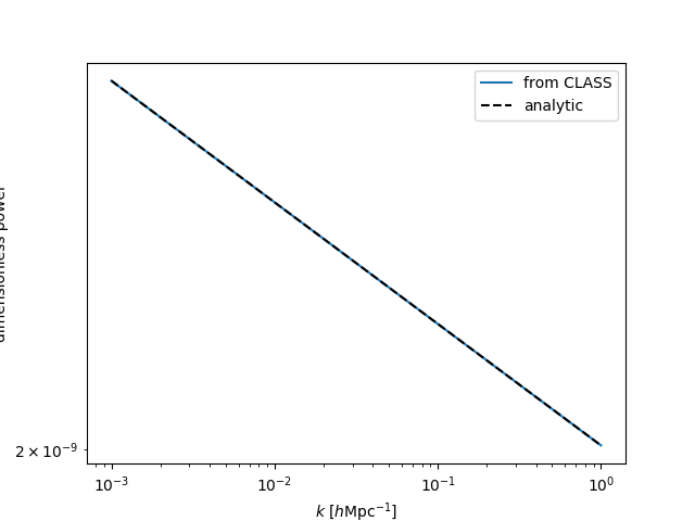
The Primordial module
The primordial module in CLASS computes
various quanitites related to the initial, primordial conditions of the Universe.
In classylss, the classylss.binding.Primordial object provides
access to the primordial power spectrum, which is defined as:
Below, we compute this quantity from the Primordial
class, and compare to the above equation:
In [82]: sp = CLASS.Spectra(cosmo)
In [83]: pm = CLASS.Primordial(cosmo)
In [84]: k = np.logspace(-3, 0, 100)
In [85]: plt.loglog(k, pm.get_pk(k), label='from CLASS')
Out[85]: [<matplotlib.lines.Line2D at 0x7fc470ecd320>]
In [86]: plt.loglog(k, sp.A_s * (k / sp.k_pivot)**(sp.n_s-1), ls='--', c='k', label='analytic')
�������������������������������������������������������Out[86]: [<matplotlib.lines.Line2D at 0x7fc4710f06a0>]
In [87]: plt.legend()
��������������������������������������������������������������������������������������������������������������Out[87]: <matplotlib.legend.Legend at 0x7fc470f39a90>
In [88]: plt.xlabel(r"$k$ $[h\mathrm{Mpc}^{-1}]$")
��������������������������������������������������������������������������������������������������������������������������������������������������������������������Out[88]: Text(0.5,0,'$k$ $[h\\mathrm{Mpc}^{-1}]$')
In [89]: plt.ylabel("dimensionless power")
�����������������������������������������������������������������������������������������������������������������������������������������������������������������������������������������������������������������������Out[89]: Text(0,0.5,'dimensionless power')